This is a guest post by Johannes Carmesin.
You have probably all heard that OpenAI announced a fully automated proof of the cycle double cover conjecture, which was conjectured independently by Tutte, Itai and Rodeh, Szekeres, and Seymour about fifty years ago.
First, to answer the most immediate question: yes, the proof is correct.
Here, I would like to do two things:
- explain the statement of the theorem; and
- give an overview of how the proof has been verified.
Statement of the theorem
The theorem has a particularly appealing topological formulation: every bridgeless multigraph can be embedded in a pseudosurface in such a way that every face is a disc. In particular, every edge occurs exactly twice among the boundary walks of the faces. Here, a pseudosurface is a topological space obtained from a closed surface (possibly disconnected) by identifying finitely many points.
The use of pseudosurfaces is very natural in this context: embeddings of different blocks can be glued together at their common cut-vertices. An example that pseudosurfaces are genuinely necessary is given below.

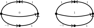
It has a unique cycle double cover. It contains each triangle twice.
The corresponding embedding has four disc faces and lies naturally in two spheres identified at the common vertex. This shows that pseudosurfaces are genuinely necessary in the topological formulation of the problem.
The algebraic counterpart of this topological statement is the following equivalent formulation: every bridgeless multigraph $G$ has a cycle double cover. That is, there exists a family $\{C_i\mid i\in I\}$ of cycles of $G$ such that every edge belongs to exactly two of the cycles $C_i$.
To see the connection, suppose first that such a cycle double cover is given. For every cycle $C_i$, take a disc and glue its boundary to the corresponding cycle in the graph. Since every edge occurs in exactly two cycles of the family, every edge is incident with two such discs. The resulting space is a pseudosurface in which the original graph is embedded and the added discs are precisely its faces.
For a simple example showing that pseudosurfaces are genuinely necessary in the above topological formulation of the cycle double cover conjecture, see the figure below.
Conversely, given such an embedding in a pseudosurface, the family $\{C_i\mid i\in I\}$ consists of the boundary walks $C_i$ of the faces of the embedding, which are cycles. Taken over all faces, these cycles form a cycle double cover, because every edge occurs exactly twice among the boundary walks of the faces.
The assumption that the graph is bridgeless is necessary. Indeed, a bridge is a cocircuit-singleton and thus cannot belong to any cycle and therefore cannot be covered even once by a cycle, let alone exactly twice.
About the proof
The proof by OpenAI establishes the second, algebraic formulation. In a nutshell, it begins with a nowhere-zero $\mathbb{F}_2^3$-flow $f$ on $G$; that is, an assignment of a nonzero vector in $\mathbb{F}_2^3$ to each edge such that, at every vertex, the values on the incident edges sum to zero. The existence of this flow follows from Seymour’s nowhere-zero six flow theorem (see also the recent short proof by DeVos and Nurse).
Roughly speaking, this flow is not quite a cycle double cover. The paper studies how one locally needs to modify the flow at each vertex so that it becomes a cycle double cover, and then there is a compatibility condition that needs to hold between adjacent vertices.
The compatibility conditions between the local modifications, and the equations for the local modifications give rise to a system of linear equations over $\mathbb{F}_2$, with one vector variable in $\mathbb{F}_2^3$ for each vertex and one scalar variable in $\mathbb{F}_2$ for each edge. OpenAI then uses duality to prove that this system always has a solution. The entire proof occupies only two pages.
Sang-il Oum gave an excellent talk on the proof and provides a much more detailed explanation. Jim Geelen (link) and Sang-il Oum (link) independently wrote short notes giving the complete proof in a different presentation, which I both find particularly pleasant to read and the latter additionally contains open questions.
Finally, the proof has already been formalised independently several times in Lean 4. Krystal Guo produced one formalisation of the core argument (personal communication), while Vaibhav Bajpai, Utku Okur, and I produced another, and one by OpenAI (see also this discussion in the AI-authored projects channel of the Lean Zulip community).