First, to answer the most immediate question: yes, the proof is correct.
Here, I would like to do two things:
explain the statement of the theorem; and
give an overview of how the proof has been verified.
Statement of the theorem
The theorem has a particularly appealing topological formulation: every bridgeless multigraph can be embedded in a pseudosurface in such a way that every face is a disc. In particular, every edge occurs exactly twice among the boundary walks of the faces. Here, a pseudosurface is a topological space obtained from a closed surface (possibly disconnected) by identifying finitely many points.
The use of pseudosurfaces is very natural in this context: embeddings of different blocks can be glued together at their common cut-vertices. An example that pseudosurfaces are genuinely necessary is given below.
The bowtie graph, consisting of two triangles glued together at a single vertex. It has a unique cycle double cover. It contains each triangle twice. The corresponding embedding has four disc faces and lies naturally in two spheres identified at the common vertex. This shows that pseudosurfaces are genuinely necessary in the topological formulation of the problem.
The algebraic counterpart of this topological statement is the following equivalent formulation: every bridgeless multigraph $G$ has a cycle double cover. That is, there exists a family $\{C_i\mid i\in I\}$ of cycles of $G$ such that every edge belongs to exactly two of the cycles $C_i$.
To see the connection, suppose first that such a cycle double cover is given. For every cycle $C_i$, take a disc and glue its boundary to the corresponding cycle in the graph. Since every edge occurs in exactly two cycles of the family, every edge is incident with two such discs. The resulting space is a pseudosurface in which the original graph is embedded and the added discs are precisely its faces.
For a simple example showing that pseudosurfaces are genuinely necessary in the above topological formulation of the cycle double cover conjecture, see the figure below.
Conversely, given such an embedding in a pseudosurface, the family $\{C_i\mid i\in I\}$ consists of the boundary walks $C_i$ of the faces of the embedding, which are cycles. Taken over all faces, these cycles form a cycle double cover, because every edge occurs exactly twice among the boundary walks of the faces.
The assumption that the graph is bridgeless is necessary. Indeed, a bridge is a cocircuit-singleton and thus cannot belong to any cycle and therefore cannot be covered even once by a cycle, let alone exactly twice.
About the proof
The proof by OpenAI establishes the second, algebraic formulation. In a nutshell, it begins with a nowhere-zero $\mathbb{F}_2^3$-flow $f$ on $G$; that is, an assignment of a nonzero vector in $\mathbb{F}_2^3$ to each edge such that, at every vertex, the values on the incident edges sum to zero. The existence of this flow follows from Seymour’s nowhere-zero six flow theorem (see also the recent short proof by DeVos and Nurse).
Roughly speaking, this flow is not quite a cycle double cover. The paper studies how one locally needs to modify the flow at each vertex so that it becomes a cycle double cover, and then there is a compatibility condition that needs to hold between adjacent vertices.
The compatibility conditions between the local modifications, and the equations for the local modifications give rise to a system of linear equations over $\mathbb{F}_2$, with one vector variable in $\mathbb{F}_2^3$ for each vertex and one scalar variable in $\mathbb{F}_2$ for each edge. OpenAI then uses duality to prove that this system always has a solution. The entire proof occupies only two pages.
Sang-il Oum gave an excellent talk on the proof and provides a much more detailed explanation. Jim Geelen (link) and Sang-il Oum (link) independently wrote short notes giving the complete proof in a different presentation, which I both find particularly pleasant to read and the latter additionally contains open questions.
This is a guest post by Donggyu Kim, who recently posted about the cycles of ribbon graphs. In this post, Donggyu introduces a generalisation of orientable ribbon graphs, pseudo-orientable ribbon graphs, based on recent work with Changxin Ding [2].
In my previous post, we saw that orientable ribbon graphs admit principally unimodular matrix representations. More precisely, for any orientable ribbon graph $\mathbb{G}$ and quasi-tree $X$, there exists a principally unimodular matrix $\mathbf{A}$ such that
$$\det(\mathbf{A}[Q \triangle X]) =\begin{cases}1 & \text{if $Q$ is a quasi-tree},\\0 & \text{otherwise},\end{cases}\qquad\qquad\tag{$*$}$$
where $Q\triangle X:= (Q\setminus X) \cup (X\setminus Q)$ denotes the symmetric difference of $Q$ and $X$, and $\mathbf{A}[Q \triangle X]$ is the principal submatrix of $\mathbf{A}$ indexed by $Q \triangle X$.
As noted in the previous post, the construction of such a matrix $\mathbf{A}$ relies heavily on the orientability of $\mathbb{G}$, and indeed it is not hard to find non-orientable ribbon graphs that do not admit such PU matrix representations.
Today, I will introduce a new class of ribbon graphs, called pseudo-orientable, which generalizes orientable ribbon graphs and admits PU matrix representations satisfying (*). For simplicity, we will restrict our attention to bouquets, that is, ribbon graphs with a single vertex. However, the results extend easily to general ribbon graphs by making use of the partial duality introduced by Chmutov [1]. We will also identify bouquets with signed chord diagrams; see Figure 1.
A bouquet (left) with three edges, where the edge $1$ is twisted/non-orientable (red) and the edges $2$ and $3$ are untwisted/orientable (blue). The corresponding signed chord diagram (right) is obtained by drawing chords on the boundary of the vertex and assigning signs (in this figure, the colors red and blue) to the chords according to the orientability of the corresponding edges.
Pseudo-orientability
Let’s begin by defining pseudo-orientable bouquets.
Definition. A bouquet $\mathbb{G}$ is pseudo-orientable if the boundary of the vertex admits two closed segments $S_1$ and $S_2$ such that
$S_1 \cap S_2$ is the set of two distinct points,
for each orientable edge, both of its ends lie in the interior of the same segment, either $S_1$ or $S_2$, and
for each non-orientable edge, one end lies in the interior of $S_1$ and the other end lies in the interior of $S_2$.
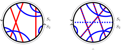
See Figure 2 (left) for an example of a pseudo-orientable bouquet.
The adjustment $\widehat{\mathbb{G}}$ of $\mathbb{G}$ at $(S_1,S_2)$ is the orientable bouquet obtained in the following way:
Cut the bouquet along $S_2$ and then reglue it with a half-twist. Note that all edges are orientable in the new bouquet.
Add a new orientable edge, denoted by $\widehat{e}$, connecting the two points in $S_1\cap S_2$.
Figure 2 (right) illustrates the resulting orientable bouquet $\widehat{\mathbb{G}}$.
The left figure is a pseudo-orientable bouquet $\mathbb{G}$, whose orientable edges are colored blue and non-orientable edges are colored red. A pair $(S_1,S_2)$ is indicated by dotted arrows. The right figure is the adjustment $\widehat{\mathbb{G}}$ of $\mathbb{G}$ at $(S_1,S_2)$, obtained by flipping the bottom segment $S_2$. The three blue-red dashed lines indicate orientable edges that were non-orientable in $\mathbb{G}$. The new edge $\widehat{e}$ is depicted as the blue dashed line. All edges in $\widehat{\mathbb{G}}$ are orientable.
Every orientable bouquet is pseudo-orientable, because we can get a pair $(S_1,S_2)$ by letting $S_1$ be a small boundary segment containing no ends of edges, and $S_2$ be the remaining boundary segment.
We also remark that the class of pseudo-orientable ribbon graphs is closed under taking ribbon graph minors.
PU matrix representations for pseudo-orientable bouquets
The Matrix–Quasi-tree Theorem for pseudo-orientable bouquets is as follows.
Theorem. Let $\mathbb{G}$ be a pseudo-orientable bouquet. Then there is an $E(\mathbb{G})$-by-$E(\mathbb{G})$ matrix $\mathbf{M}$ such that
$$\det(\mathbf{M}[Q])=\begin{cases}1 & \text{if $Q$ is a quasi-tree},\\0 & \text{otherwise}.\end{cases}$$
In particular, $\det(\mathbf{I} + \mathbf{M})$ is the number of quasi-trees of $\mathbb{G}$.
Remarkably, the matrix $\mathbf{M}$ is neither skew-symmetric nor symmetric in general, but can be expressed as the sum of a skew-symmetric matrix and a rank-one symmetric matrix. The theorem follows from two parallel stories on ribbon graphs and matrices, with delta-matroids underlying both.
For a subset $S$ of $[n]:=\{1,2,\ldots,n\}$, let
$$\widehat{S} :=\begin{cases}S & \text{if $|S|$ is even},\\S\cup\{n+1\} & \text{if $|S|$ is odd}.\end{cases}$$
Ribbon graphs. Let $\mathbb{G}$ be a pseudo-orientable bouquet, and let $\widehat{\mathbb{G}}$ be an adjustment of $\mathbb{G}$. We set $E(\mathbb{G}) = [n]$ and $\widehat{e} = n+1$. Then the following equivalence holds:
$$\text{$Q$ is a quasi-tree of $\mathbb{G}$} \iff \text{$\widehat{Q}$ is a quasi-tree of $\widehat{\mathbb{G}}$}.\tag{1}$$
Matrices. Let $\mathbf{A}$ be an $(n+1)$-by-$(n+1)$ PU skew-symmetric matrix representing $\widehat{\mathbb{G}}$. We can write it as
By the property (*) of the matrix $\mathbf{A}$ representing $\widehat{\mathbb{G}}$ (with $X=\emptyset$) together with (1) and (2), we deduce the theorem.
Delta-matroids. Delta-matroids are already lurking in the two pictures above. Recall that a ribbon graph gives rise to a delta-matroid via its quasi-trees, and a (skew-)symmetric matrix gives rise to a delta-matroid via the index sets of nonsingular principal submatrices. Moreover, the delta-matroid associated with an orientable ribbon graph is even. What, then, can we say about the delta-matroid associated with a pseudo-orientable ribbon graph?
A delta-matroid $D$ is strong if it satisfies the simultaneous basis exchange property: for any bases $B,B’$ and $x\in B\triangle B’$, there is $y\in B\triangle B’$ such that $B\triangle\{x,y\}$ and $B’\triangle\{x,y\}$ are bases.
Every matroid, even delta-matroid, and ribbon-graphic delta-matroid is strong, but not every delta-matroid is. For example, the delta-matroid $([3],\{\emptyset,\{1\},\{2\},\{3\},\{1,2,3\}\})$ is not strong.
Murota [4] gave a concise relationship between strong and even delta-matroids, attributing it to Geelen:
Proposition. Let $D = ([n],\mathcal{B})$ be a set system. Then $D$ is a strong delta-matroid if and only if $\widehat{D} := ([n+1],\widehat{\mathcal{B}})$ is an even delta-matroid, where $\widehat{\mathcal{B}} := \{ \widehat{B} : B\in\mathcal{B} \}$.
Finally, pseudo-orientable ribbon graphs are precisely those ribbon graphs $\mathbb{G}$, up to ribbon graph $2$-isomorphism [3], for which $\widehat{D(\mathbb{G})}$ is ribbon-graphic — this characterization captures our original motivation for the study [2].
Acknowledgements
I thank Changxin Ding and Jorn van der Pol for helpful comments.
References
[1] Sergei Chmutov. Generalized duality for graphs on surfaces and the signed Bollobas–Riordan polynomial. J. Combin. Theory Ser. B 99(3):617–638, 2009. doi:10.1016/j.jctb.2008.09.007 [2] Changxin Ding and Donggyu Kim. Pseudo-orientable ribbon graphs: Matrix–Quasi-tree theorem and log-concavity, 2026. arXiv preprint. [3] Iain Moffatt and Jeaseong Oh. A 2-isomorphism theorem for delta-matroids. Adv. in Appl. Math. 126, Paper No. 102133, 2021. doi:10.1016/j.aam.2020.102133 [4] Kazuo Murota. A note on M-convex functions on jump-systems. Discrete Appl. Math. 289:492–502, 2021. doi:10.1016/j.dam.2020.09.019
This is a guest post by Donggyu Kim, who discusses the cycles of an embedded graphs (ribbon graphs) and their interactions with the associated delta-matroids. It is based on joint work with Matt Baker and Changxin Ding [1].
Ribbon graphs and quasi-trees
An embedded graph $G$ is a graph cellularly embedded in a closed (possibly non-orientable) surface $\Sigma$. We think of vertices and edges as disks and rectangles, obtained by thickening the points and lines by a sufficiently small $\epsilon>0$ in the surface $\Sigma$. In this sense, embedded graphs are often called ribbon graphs; we will use the two notions interchangeably.
A typical example of an embedded graph is a connected plane graph – but instead of embedding the graph in the plane, let’s embed it on the sphere! One easy exercise is that a spanning subgraph $T$ is a spanning tree if and only if it, viewed as a ribbon graph, has a unique boundary component. However, these two notions diverge when the surface $\Sigma$ is not the sphere. Every spanning tree has a unique boundary component, but the converse doesn’t hold. We call a spanning subgraph with a unique boundary component a quasi-tree. The figure below depicts an embedded graph on the torus $\mathbb{T}^2$; it has a quasi-tree that is not a spanning tree. Since quasi-trees capture topological information, they are the right analog of spanning trees for embedded graphs.
Figure 1. A plane graph (an embedded graph on the sphere $\mathbb{S}^2$, left) and the corresponding ribbon graph (middle). The spanning subgraph with edge set $\{1,4,5\}$ (top right) has a unique boundary component as a ribbon graph, whereas the spanning subgraph with edge set $\{1,2,5\}$ (bottom right) has three boundary components – don’t miss the boundary of the degree-$0$ vertex.
Ribbon cycles
Question. We have seen that quasi-trees are the right analog of spanning trees for embedded graphs. What should play the role of cycles?
Before answering the question, let’s fix a convention. Since we’ll only care about the topological properties – such as whether $\Sigma – H$ is connected for a subgraph $H$ (we’ll make this more precise below) – every subgraph in this post will be assumed to be spanning (i.e., containing all vertices of the original graph). Hence, we will identify an edge set with the corresponding spanning subgraph. Moreover, we may view $\Sigma – H$ either as removing $H$ as a graph or as a ribbon graph. These two viewpoints are homeomorphic, so the reader may adopt whichever is more convenient.
With this convention in place, let’s return to the plane case (Figure 1). For any cycle $C$, the surface $\Sigma – C$ is disconnected; indeed, the cycles are exactly the minimal subgraphs with this property. What happens for general embedded graphs? Consider Figure 2. Even after removing any cycle from the torus $\mathbb{T}^2$, it remains connected. Moreover, there is no subgraph $H$ for which $\Sigma – H$ is disconnected.
Figure 2. A graph embedded on the torus (left) and the corresponding ribbon graph (right). It has four quasi-trees with edge sets $\{1\}$, $\{2\}$, $\{3\}$, and $\{1,2,3\}$.
Ordinary cycles alone cannot be the right answer on a general surface. To fix this, we need to bring the dual graph into the picture. Let us draw both the graph $G$ embedded on the torus, shown in Figure 2, and its geometric dual $G^*$ simultaneously; see Figure 3. The graph $G$ is drawn in black, and the dual $G^*$ is drawn in red. We can then separate the torus $\mathbb{T}^2$ into two components by removing a cycle $\{1,2\}$ of $G$ together with a cycle $\{3^*\}$ of $G^*$.
Figure 3. The embedded graph $G$ in Figure 2 together with its dual $G^*$. It has four ribbon cycles: $\{1,2,3^*\}$, $\{1,2^*,3\}$, $\{1^*,2,3\}$, and $\{1^*,2^*,3^*\}$.
Denote $E:=E(G)$ and $E^*:= E(G^*) = \{e^*:e\in E\}$. A subset $S \subseteq E\cup E^*$ is a subtransversal if it contains at most one of $e$ or $e^*$ for each edge $e\in E$.
Definition. Let $G$ be an embedded graph on $\Sigma$. A ribbon cycle of $G$ is a subtransversal $C \subseteq E\cup E^*$ that minimally separates the surface $\Sigma$, meaning that $\Sigma – C$ is disconnected while $\Sigma – C’$ is connected for every $C’\subsetneq C$.
If $G$ is a plane graph, then the ribbon cycles are exactly the cycles and the stars of bonds. For example, the ribbon cycles of the plane graph in Figure 1 (see also Figure 4) are
$\{1,2,5\}$, $\{3,4,5\}$, $\{1,2,3,4\}$, $\{1^*,2^*\}$, $\{3^*,4^*\}$, $\{1^*,3^*,5^*\}$, $\{1^*,4^*,5^*\}$, $\{2^*,3^*,5^*\}$, and $\{2^*,4^*,5^*\}$.
Figure 4. The plane graph in Figure 1 (black) and its geometric dual (red).
The embedded graph on the torus in Figure 3 has four ribbon cycles:
$\{1,2,3^*\}$, $\{1,2^*,3\}$, $\{1^*,2,3\}$, and $\{1^*,2^*,3^*\}$.
Each ribbon cycle $C$ is a union of cycles in $G$ and cycles in $G^*$. In other words, $C\cap E$ forms an Eulerian subgraph of $G$, and $C\cap E^*$ forms an Eulerian subgraph of $G^*$. The ribbon cycle $\{1^*,2^*,3^*\}$ consists of three cycles – $\{1^*\}$, $\{2^*\}$, and $\{3^*\}$ – which share a common vertex.
The following is an amusing exercise, a counterpart of the orthogonality of cycles and bonds in ordinary graphs. For an edge $e$ of an embedded graph $G$, we denote $(e^*)^* = e$, and write $C^* := \{e^* : e\in C\}$ for any subset $C\subseteq E\cup E^*$.
Exercise (Orthogonality). Let $C_1$ and $C_2$ be two ribbon cycles of $G$. Then $|C_1\cap C_2^*| \ne 1$.
Circuits of ribbon-graphic delta-matroids
Now that we have a topological candidate for the “cycles” of a ribbon graph, the next question is whether the delta-matroid associated with the ribbon graph captures the same objects. Carolyn Chun explained earlier that the quasi-trees of an embedded graph $G$ form the bases of a delta-matroid, denoted $D(G)$.
A graph gives rise to its graphic matroid in (at least) two familiar ways: by collecting maximal acyclic sets, we obtain the bases; by collecting cycles, we obtain the circuits. Thus one may ask whether the ribbon cycles of an embedded graph $G$ are the circuits of $D(G)$. However, there are two hurdles. First, the ground sets do not match, $E$ vs. $E\cup E^*$. Second, the bases of a delta-matroid are not equicardinal—which raises a problem, since bases cannot in general be recovered from circuits if the circuits are defined as minimal subsets not contained in any basis.
These issues can be easily resolved by introducing symmetric matroids [2] (also known as 2-matroids; see Irene Pivotto’s post), which are a homogenized version of delta-matroids.
Let $D = (E,\mathcal{B})$ be a finite set system. Then $D$ is a delta-matroid if and only if $\mathrm{lift}(D) := (E\cup E^*, \mathcal{B}’)$ is a symmetric matroid, where $\mathcal{B}’ := \{B\cup (E\setminus B)^* : B\in \mathcal{B}\}$. Since all bases of a symmetric matroid have the same cardinality, it makes sense to define its circuits. A circuit of a symmetric matroid is a minimal subtransversal that is not contained in any basis.
Now we can state the following:
Theorem. The circuits of $\mathrm{lift}(D(G))$ are exactly the ribbon cycles of an embedded graph $G$.
To prove this, let us first see equivalent characterizations of quasi-trees. Recall that a quasi-tree $Q$ is a spanning subgraph with a unique boundary component. Hence, $\Sigma-Q$ also has a unique boundary component, which implies that $\Sigma-Q$ is connected. The following folklore result says that an even stronger statement holds.
Proposition. For $Q\subseteq E(G)$, the following are equivalent:
$Q$ is a quasi-tree of $G$.
$(E\setminus Q)^*$ is a quasi-tree of the dual $G^*$.
$\Sigma – Q – (E\setminus Q)^*$ is connected.
We also note the following corollary orthogonality.
Exercise. For any subtransversal $S\subseteq E\cup E^*$ such that $\Sigma – S$ is connected, there is a transversal $T$ (that is, a subtransversal of size $|E|$) containing $S$ such that $\Sigma – T$ is still connected.
Hence, quasi-trees $Q$ can be identified with “maximal subtransversals $Q\cup (E\setminus Q)^*$ whose removal does not disconnect the surface,” whereas ribbon cycles are “minimal subtransversals whose removal disconnects the surface.” This proves the theorem above. Great! Ribbon cycles really are the right circuit-like objects.
Representations of ribbon-graphic delta-matroids via signed ribbon cycles
A natural next question is whether other familiar graph/matroid correspondences also survive in the ribbon-graph world. For example, if $G$ is an ordinary connected graph with an arbitrary orientation, we can quickly find a regular representation of $M(G)$ by examining the fundamental bonds with respect to a spanning tree:
Fix a spanning tree $T$.
For each $e\in E(T)$, let $C_e$ be the unique bond in the complement of $T-e$, called the fundamental bond of $e$ with respect to $T$.
Since a reference orientation of $G$ is given, we can identify $C_e$ with a $(0,\pm 1)$-vector (of course, this is determined up to sign, and we may choose either sign).
Construct a real $(|V|-1)$-by-$|E|$ matrix $\mathbf{A}$ by taking the vectors $C_e$ as its rows.
Then $\mathbf{A}$ is a totally unimodular matrix representing $M(G)$. In the same way, one can construct a totally unimodular matrix representing $M^*(G)$ by examining the fundamental cycles.
Remarkably, almost the same construction works for “orientable” ribbon graphs. Fix one of the two orientations of $\Sigma$. Here we choose the counterclockwise orientation with respect to normal vectors, the so-called right-hand rule. Fix a reference orientation for $G$. Then we can assign the corresponding dual reference orientation to $G^*$; see the figure below.
Figure 5. For each oriented edge $e$, we assign the dual orientation of $e^*$ as depicted on the left. The illustration on the right shows a reference orientation of $G$ in Figure 3 together with the corresponding dual reference orientation of $G^*$.
The point of the next four steps is to construct a matrix representing $\mathrm{lift}(D(G))$ from signed ribbon cycles.
Fix a quasi-tree $Q$. Denote $B := Q\cup (E\setminus Q)^*$.
For each $e \in E(G)$, let $C_e$ be the ribbon cycle in $B\triangle\{e,e^*\}$, which always exists and is unique!
We identify $C_e$ with a $(0,\pm 1)$-vector $\mathbf{v}_e$ in $\mathbb{R}^{E\cup E^*}$ defined as follows:
$\Sigma-C_e$ separates the surface into two components. Choose one of them, say $\Sigma’$.
$C_e$ is exactly the boundary of $\Sigma’$. Because $\Sigma’$ is oriented, we obtain a $(0,\pm 1)$-vector $\mathbf{v}_e$ supported on $C_e$ by setting \[\mathbf{v}_e(f) =\begin{cases}+1 & \text{if the orientation of $f\in C_e$ agrees with that of $\Sigma’$}, \\-1 & \text{if the orientation of $f\in C_e$ is opposite to that of $\Sigma’$}, \\0 & \text{if $f\notin C_e$}.\end{cases}\]
Construct a real $|E|$-by-$2|E|$ matrix $\mathbf{A}$ by taking the vectors $\mathbf{v}_e$ as its rows.
Proposition. Let $X$ be a transversal of $E\cup E^*$. Then $X \cap E$ is a quasi-tree of $G$ if and only if the $|E|$-by-$|E|$ submatrix $\mathbf{A}[(E\cup E^*) \setminus X]$ with columns $(E\cup E^*) \setminus X$ is nonsingular; in fact, its determinant is $\pm 1$.
Let’s see an example in the following figure.
Figure 6. Choose a quasi-tree $Q = \{1,2,3\}$. Then the ribbon cycles defined in Step 2 are $C_1 = \{1^*,2,3\}$ (left), $C_2 = \{1,2^*,3\}$ (middle), and $C_3 = \{1,2,3^*\}$ (right). The removal of each ribbon cycle $C_i$ from the torus $\mathbb{T}^2$ disconnects it into two components. In Step 3(a), we color $\Sigma’$ yellow.
The vectors $\mathbf{v}_i$ defined in Step 3(b) are
The entries in the first row are indexed by $1,2,3$ from left to right, and the entries in the second row are indexed by $1^*,2^*,3^*$ from left to right. Thus, the resulting matrix $\mathbf{A}$ in Step 4 is
where the columns are indexed by $1,2,3,1^*,2^*,3^*$ in this order. You can check that the matrix $\mathbf{A}$ satisfies the proposition.
After multiplying some rows by $-1$ and rearranging the columns, the matrix $\mathbf{A}$ in the proposition can be written as a matrix of the form $\left( \begin{array}{c|c} \mathbf{I}_n & \mathbf{S} \end{array} \right)$, where $\mathbf{I}_n$ is the identity matrix with size $n:=|E|$ and $\mathbf{S}$ is a principally unimodular skew-symmetric matrix. An equivalent construction of $\mathbf{S}$ was first given by Bouchet [2] in terms of (principally) unimodular orientations of circle graphs. If you are curious about the relationship between the above matrix construction and Bouchet’s construction, see Appendix A of [1]. Merino, Moffatt, and Noble [3] pointed out that
\[\det(\mathbf{I}_n + \mathbf{S}) = \# \text{quasi-trees of $G$},\]
The above matrix construction depends strongly on the orientability of the surface. This appears explicitly in Step 3, where we choose the signs of the entries of the $(0,\pm 1)$-vector $\mathbf{v}_e$. It is also implicit in Step 2, since we cannot guarantee the existence of $C_e$ when the surface is non-orientable.
Question. How about non-orientable ribbon graphs? Could we also obtain nice representations by unimodular matrices?
The short answer is: yes for some non-orientable ribbon graphs, but not for every ribbon graph. I will continue this discussion in the next post. See you then!
Acknowledgements. I thank Matt Baker, Changxin Ding, and Jorn van der Pol for helpful comments.
References
[1] Matthew Baker, Changxin Din, and Donggyu Kim. The Jacobian of a regular ortogonal matroid and torsor structures of quasi-trees of ribbon graphs, 2025. arXiv preprint.
[2] André Bouchet. Greedy algorithm and symmetric matroids. Math. Program. 38(2):147–159, 1987. doi:10.1007/BF02604639.
[3] Criel Merino, Iain Moffatt, and Steven Noble. The critical group of a combinatorial map. Comb. Theory 5(3), paper no. 2, 41, 2025. doi:10.5070/C65365550.
A $q$-analog is formed by replacing the notion of a set by the notion of a vector space, with a corresponding replacement of other concepts: cardinality becomes dimension, elements are replaced by 1-dimensional subspaces, the empty set is replaced by the 0-dimensional subspace, intersection remains the same, and union is replaced by sum. (It is not always clear how to replace set difference or symmetric difference.) The application of this idea to matroid theory gives the theory of q-matroids [Jur2018][Cer2022], which Relinde Jurrius has described in this forum, most recently with the analog of delta-matroids. In this post I’ll define a $q$-analog of a transversal [Mir1971], and show that there is still a connection with matroids, as well as analogs of many of the main theorems of transversal theory. A more complete account has been posted on arXiv.
$q$-matroids, briefly
A $q$-matroid can be characterized by its bases, independent sets, circuits, or spanning sets, but the simplest definition for our purposes is via the rank function.
Definition 0. Let $V$ be a vector space and ${\cal L}(V)$ be the lattice of subspaces of $V$. A $q$-matroid on $V$ is determined by a rank function $r: {\cal L}(V) \rightarrow \mathbb{Z}$, satisfying, for all $A, B \in {\cal L}(V)$,
$0 \leq r(A) \leq \dim A$ (rank is non-negative and bounded by dimension),
if $A \leq B$ then $r(A) \leq r(B)$ (rank is non-decreasing), and
$r(A \vee B) + r(A \wedge B) \leq r(A) + r(B)$ (rank is submodular).
The usual concepts of matroid theory apply equally well to $q$-matroids: a subspace $A$ is independent if $r(A) = \dim A$, and dependent otherwise; a subspace $A$ is a circuit if it is dependent but all its proper subspaces are independent; the closure of $A$ is the largest subspace $B$ with $A \leq B \leq V$ and $r(B) = r(A)$; and $A$ is spanning if its closure is $V$. Axiom systems for $q$-matroids in terms of independent sets, bases, or circuits can be found in [Cer2022].
The closure of the trivial subspace $\{ 0 \}$ gives the so-called loop space of the matroid; any subspace of rank 0 is contained in this loop space. A $q$-matroid of rank 1 is therefore completely characterized by its loop space $L$, with the rank of a subspace $X$ being 0 if it is a subspace of $L$ and 1 otherwise.
A large class of $q$-matroids can be defined algebraically; these are the representable $q$-matroids. Given some $n\times m$ matrix $G$ over a field $K$ extending $\mathbb{F}_q$, we can define the $q$-matroid represented by $G$ as follows: if a subspace of $\mathbb{F}_q^m$ is the row space of matrix $X$, then its rank in the $q$-matroid is the rank of $GX^T$. It can be seen that this does not depend on the matrix $X$ we use; if $X$ and $Y$ are full-rank matrices with equal row spans, then there is some invertible matrix $A$ so that $Y = AX$. Then $GY^T = GX^TA^T$, and as $A^T$ is invertible, the ranks are the same. Note that the entries of $G$ may lie in a larger field than the vector space is defined over. Usually $K$ is equal to $\mathbb{F}_{q^k}$ for some $k$.
Unlike a normal matroid that might be representable over fields of many different characteristics, a $q$-matroid representation has its characteristic fixed by the vector space the $q$-matroid is defined on. I suppose the interesting question about representations is then which extension fields are possible.
Normal transversals, abnormally
To have a clear connection to $q$-matroids, it seems to work best to analogize a cryptomorphic version of transversal theory. Where the usual definition has membership, this definition uses non-membership.
Definition Given an indexed family ${\cal X} = (X_1,X_2, \dotsc, X_n)$ of subsets of some given set $S$, an avoiding transversal of $\cal X$ is a set of elements $x_1, x_2, \dotsc, x_n$ of $S$, all distinct, with each $x_i \notin X_i$. A partial avoiding transversal of $\cal X$ is an avoiding transversal of some subfamily (that is, containing some subset of the $X_i$).
Clearly, when $A_i = S \setminus X_i$, an avoiding transversal of $\cal X$ is just a transversal of the $A_i$.
The main properties of transversals can be recast in this setting. We first define ${\cal X}(J) = \bigcap_{j\in J} X_j$ for any $J \subseteq \{1, 2, \dots,n\}$, with the convention ${\cal X}(\emptyset) = S$.
Theorem
(Hall) $\cal X$ has a transversal iff for all $J \subseteq \{1, 2, \dots,n\}$ we have $|{\cal X}(J)| + |J| \leq |S|$.
(Rado) Suppose $M$ is a matroid on $S$ with co-nullity function $\nu^*$. $\cal X$ has a transversal that is independent in $M$ iff for all $J \subseteq \{1, 2, \dots,n\}$ we have $\nu^*({\cal X}(J)) + |J| \leq \nu^*(S)$.
(Edmonds and Fulkerson) The set of partial transversals of $\cal X$ are the independent sets of a matroid.
(Piff and Welsh) Transversal matroids are representable over every sufficiently large field.
A matroid is transversal iff it is the union of a collection of rank-1 matroids.
When $M$ is the matroid whose independent sets are the partial avoiding transversals of $\cal X$ we say that $M$ is a transversal matroid and $\cal X$ is a co-presentation of $M$. Co-presentations have some nice properties:
If the rank of transversal matroid $M$ is $r$, then $M$ has a co-presentation with $r$ elements.
If $\cal X$ is a co-presentation of $M$ and the rank of $M$ is $r$, then $\cal X$ has a subfamily with $r$ elements that is also a co-presentation of $M$.
If $(X_1, \dots, X_r)$ is a co-presentation of $M$, then each $X_i$ is a flat.
If $M$ is a transversal matroid, then it has a unique minimal co-presentation, where a co-presentation is minimal if no members can be removed or replaced by strictly smaller sets while still co-representing $M$.
$q$-transversals, finally
In this section we will be talking about the vector space $V$ and its subspaces as well as $q$-matroids, so there is room for some confusion when we say “independent” or “basis”. Therefore we will qualify these terms and speak of a “vector basis” or “independent vectors” when referring to $V$ and its elements, or a “matroid basis” or “independent subspace” when referring to aspects of a $q$-matroid.
Definition Let a vector space $V$ be given, together with a family ${\cal X} = (X_1, \dotsc, X_n)$ of subspaces of $V$. A $q$-transversal is a dimension $n$ subspace $T$ of $V$ where every vector basis $B$ of $T$ has an ordering $B = \{b_1, \dots, b_n\}$ such that $b_i \notin X_i$ for $i \in\{1,2,\dotsc,n\}$. That is, every vector basis of $T$ is an avoiding transversal of $\cal X$. A partial $q$-transversal is a dimension $n$ subspace $T$ where every vector basis of $T$ is a partial avoiding transversal of $\cal X$.
The definition of partial $q$-transversal deserves some note. It would be more analogous to the conventional theory to declare a partial $q$-transversal to be a $q$-transversal of some subsystem of $\cal X$. This turns out to be equivalent, but is more difficult to work with. Analogs of the major properties of transversals are also enjoyed by $q$-transversals as defined this way:
Theorem
Family $\cal X$ has a $q$-transversal iff for every nonempty $J \subseteq \{1, 2, \dots, n\}$ we have $\dim {\cal X}(J) + |J| \leq \dim V$.
The set of partial $q$-transversals of a family form the independent subspaces of a $q$-matroid.
A $q$-matroid is $q$-transversal iff it is the union of a collection of rank 1 $q$-matroids.
I conjecture that all $q$-transversal matroids are representable, but have only proven a special case where the spaces $X_i$ align is a particular way:
Theorem Suppose that $V$ has a vector basis $\{b_1, b_2, \dotsc, b_n\}$ so that each of the $X_i$ has the form $X_i = \left< b_i \,|\, i \in L_i \right>$ for some sets $L_i \subseteq \{1, 2, \dots, n \}$. Then the associated $q$-transversal matroid is representable.
I also conjecture that an analog of Rado’s theorem holds. Recall that if $\cal B$ is the set of bases of matroid $M$, then co-nullity satisfies $\nu^*(X) = \min_{B \in \cal B} | B \cap X |$, so we may plausibly define a $q$-analog $\bar n$ satisfying $\bar n(X) = \min_{B \in \cal B} \dim(B \wedge X)$ for a $q$-matroid $M$ with bases $\cal B$.
Conjecture Suppose $M$ is a $q$-matroid on vector space $V$, with rank function $r$, and $\cal X$ is a system of subspaces of $V$. Then $\cal X$ has a $q$-transversal that is independent in $M$ iff for all $J \subseteq I$ we have $\bar n ({\cal X}(J)) + |J| \leq \bar n (V)$.
When $M$ is the $q$-matroid whose independent spaces are the set partial $q$-transversals of a family $\cal X$ we say that $M$ is $q$-transversal and that $\cal X$ is a presentation of $M$.
If the rank of $q$-transversal matroid $M$ is $r$, then $M$ has a presentation with $r$ elements.
If $\cal X$ is a presentation of $q$-matroid $M$ and the rank of $M$ is $r$, then $\cal X$ has a subfamily with $r$ elements that is also a presentation of $M$.
If $(X_1, \dots, X_r)$ is a presentation of $M$, then each $X_i$ is a flat.
I conjecture that any $q$-transversal matroid has a unique minimal presentation.
As can be seen, while there are still some interesting questions to be settled, the analogy with normal transversal theory looks promising. Details and proofs are in the paper on arXiv [Saa2025].
References
[Cer2002] Michela Ceria and Relinde Jurrius. Alternatives for the $q$-matroid axioms of independent spaces, bases, and spanning spaces.arXiv.org/abs/2207.07324v3, December 2022.
[Jur2018] Relinde Jurrius and Ruud Pellikaan. Defining the $q$-analog of a matroid.Article #P3.2, The Electronic Journal of Combinatorics 25(3), 2018.
[Mir1971] Leon Mirsky. Transversal Theory: an account of some aspects of combinatorial mathematics. Academic Press, 1971.